Complex Numbers
Overview
1 | What are complex numbers?
1.1 The need for complex numbers
we require the set of integers, \(\mathbb{Z} = \{0, \pm1, \pm2, \pm3,...\}\). However, we soon run into problems with decimals, such as
The set of rational numbers, \(\mathbb{Q}\), which are numbers expressed as a fraction of two integers, is needed. Once we begin to involve exponents in our equations, such as in
which is when complex numbers save the day.
2 | Definitions
The fundamental theorem of algebra states that, for a complex polynomial \(p_n(z)\) of degree n, the equation \(p_n(z)\) = 0 has precisely n complex roots. Complex numbers, \(\mathbb{C}\), include all sets of numbers mentioned previously, plus the set of imaginary numbers. Therefore, with complex numbers, the set of numbers is algebraically closed.
A complex number is most often written as a sum of a real part and imaginary part,
in which \(x, y \in \mathbb{R}\) and \(i = \sqrt{-1}\) is an imaginary unit.
The real part of z is written as \(Re\{z\} = x\) and the imaginary part of z is written as \(Im\{z\} = y\).
Each complex number has a complex conjugate, in which the imaginary part is negated. The complex conjugate of the complex number z written above is
What would happen if we were to take powers of \(i\)?
Power of \(i\) |
in numbers please |
|---|---|
\(i^{-1}\) |
\(-\sqrt{-1}\) |
\(i^0\) |
\(1\) |
\(i^1\) |
\(\sqrt{-1}\) |
\(i^2\) |
\(-1\) |
\(i^3\) |
\(-\sqrt{-1}\) |
\(i^4\) |
\(1\) |
\(i^5\) |
\(\sqrt{-1}\) |
With four additional powers, we managed to return right back to the start. This is equivalent to rotating 90º four times on a geometric plane…
2 | Visualizing complex numbers
2.1 The complex plane
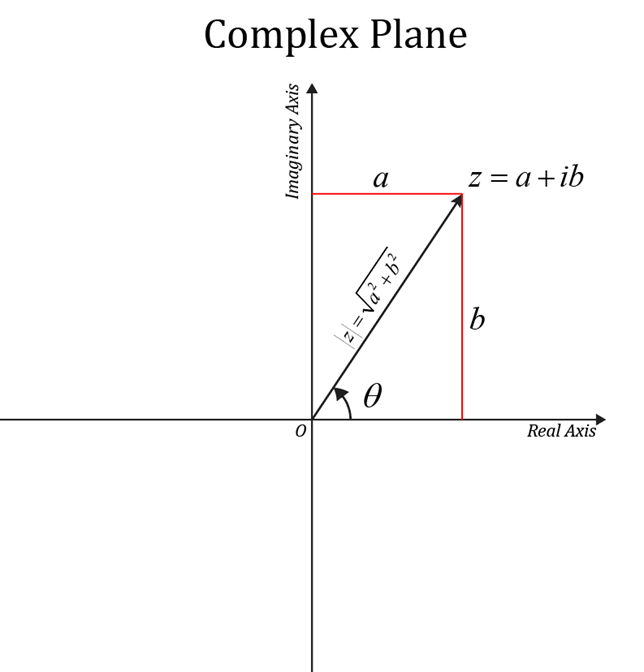
The real and imaginary parts of a complex number are orthogonal, such that they form a two-dimensional plane refered to as the complex plane.
A complex number is represented as a vector pointed a distance outwards from the origin \((0,0)\), with the real part the distance along the x-axis, and the imaginary part the distance along the y-axis.
2.2 Polar coordinates
Complex numbers can easily be visualized with both cartesian and polar coordinates. The magnitude of the vector formed by a complex number z in the complex plane, or the modulus of the complex number, is
and the angle from the real axis (counterclockwise) is the argument of the complex number,
Therefore, a complex number can be represented with a radius \(r\) and an angle \(\theta\), called polar form, instead of two distances, \(x\) and \(y\), called cartesian form, like
The argument is actually infinitely many values, as it includes a principal argument plus any integer multiplied by \(2\pi\),
where \(n = \{0, \pm1, \pm2, \pm3,...\}\). The principal argument \(Arg(z)\) is the value defined within some specified bounds, such as \(-\pi<\theta<\pi\) or \(0<\theta<2\pi\).
2.3 Euler’s formula
Essential to operating on complex numbers is Euler’s formula:
We now have three ways to write the same complex number:
The different forms have different benefits that will be explored in the following sections.
The unit circle becomes a very helpful tool when solving problems involving complex numbers.
3 | Operating on complex numbers
3.1 Addition and Subtraction
To add or subtract two complex numbers, it is best to add their real and imaginary parts separately, like
or
3.2 Multiplication
To multiply two complex numbers, use FOIL (first outer inner last) on two numbers in cartesian form to multiply each pair:
Alternatively, complex numbers in exponential polar form can be multiplied when both their moduli are multiplied and their arguments are added together:
3.3 Division
To divide one complex number by another, multiply the numerator and denominator by the complex number of the divisor.
This avoids having a complex number in the denominator.
Alternatively, complex numbers in exponential polar form can be divided when the modulus of the dividend is divided by that of the divisor and the argument of the divisor is subtracted from that of the dividend:
3.4 Powers
It is easiest to take powers of complex numbers when they are in exponential polar form. The \(n\)th power of a complex number is
3.5 Roots
Taking the \(n\)th root of a complex number is a little trickier. The finding the modulus is light work, as \(|z^{\frac{1}{n}}| = r^{\frac{1}{n}}\). But there are \(n\) distinct roots of a complex number, forming a polynomial with \(n\) vertices, each a distance of \(r^{\frac{1}{n}}\) from the origin.
First, define the range of values for the arguments. Then, find the \(n\) distinct roots by adding multiples of \(2\pi\) divided by \(n\) to the prinicpal argument.
where \(k = \{0, \pm1, \pm2, \pm3,...\}\).
4 | References
Riley Hobson and Bence (2006). Mathematical Methods for Physics and Engineering, 3rd Edition.
MATH 120A notes by Professor Rabin
Ashton Domi’s 2024 Complex Numbers Lecture
Merino, O. (2006). “A Short History of Complex Numbers.” University of Rhode Island.
5 | Appendix
5.1 Comparing complex numbers
There is no method to compare two complex numbers directly. For example, if \(z_1\) and \(z_2\) are complex numbers and \(z_1 \neq z_2\), then \(z_1 < z_2\) or \(z_1 > z_2\) cannot be defined (\(i<0\) and \(i<0\) are both untrue statements when squared).
The triangle inequality avoids this complication by comparing the moduli of two complex numbers, and is true for n complex numbers:
The law of cosines only applies to two complex numbers:
Here, \(\cos(\phi)\) is bounded by -1 and +1.
5.2 A brief history of complex numbers
According to a review by Orlando Merino, “A Short History of Complex Numbers” (2006), the need for complex numbers arose from solving cubic equations, instead of quadratic equations.
Al-Khwarizmi (780-850), a scientist of Baghdad, was one of the first to find geometric-based solutions to quadratics, but would only consider the positive roots. When Arabic methods traveled to Italy, Leonardo da Pisa (streetname Fibonacci, 1170-1250), was able to perform for the emperor the solutions to many cubic equations.
Gerolamo Cardano’s friend Antonio Maria Fiore wins a math battle and shares his secrets from his teacher Scipione del Ferro with him. Cardano was able to back out the winning formula and published it in “Ars Magna” (1545). The book featured complex numbers of the form \(a + \sqrt{-b}\), of which Cardano wrote as being “mental tortures” to deal with.
Later, Rafael Bombelli finds the imaginary unit, \(\sqrt{-1}\) in “l’Algebra” (1572, 1579) and calles it “più di meno.”
René Descarts (1596-1650) coins the term imaginary, John Wallis (1616-1703) comes later with the geometric interpretation of i, and Euler (1707-1783) drops the banger \(e^{i\theta}= \cos(\theta) + i\sin(\theta)\).
[ ]: