Linear Algebra 1
Instructor: Tommy Stone, Applied Ocean Science (AOS) PhD student (thstone@ucsd.edu)
TAs: Sam Schulz (s1schulz@ucsd.edu), Camilla Marcellini (cmarcellini@ucsd.edu )
Linear algebra is a branch of mathematics that studies vectors, vector spaces, linear transformations, and systems of linear equations. At its core, it provides a framework for understanding and working with quantities that have both magnitude and direction, as well as the relationships between them. The subject focuses on operations with matrices and vectors, making it a powerful language for expressing and solving mathematical problems.
Lecture notes adapted from
David Vishny 2022 lecture notes for the SIO Math Workshop
Essence of Linear Algebra By 3Blue1Brown
Linear Algebra and Its Applications by Gilbert Strang, 4th Edition
Mathematical Methods for Physics and Engineering By K.R Riely, M.P Hobson, S. J. Bence
1 | Why Linear Algebra?
The first question we must ask is why is Linear Algebra important in Earth Sciences?
1.1 Application of Linear Algebra
Linear Algebra is essential because it provides the mathematical foundation for analysis of large datasets, solving a system of equations as well as identifying patterns in complex systems. Earth Science disciplines use Linear Algebra with General Circulation Models (CGM), Wave Dynamics, Eigenvalues, Singular Value Decomposition (SVD), Least Squares Fitting, Neural Networks and many more. In order to go into these advanced topics we need to first to learrn the basis of Linear Algebra which are vectors and matrices.
2 | Review - Scalars, Vectors, Matrices, Tensors and Dimensions (Oh my!)
In this first section we will review our definitions of
Scalars
Vectors
Matrices
Tensors
2.1 Notation
Typical notation you will find for scalars, vectors and matrices
Scalars are indicated by lower case letters.
Vectors will have an arrow above a lower case letter
Another way to represent a vector is by multiplying the scalar values of \(u_x,u_y,u_z\) by their basis vectors \(\hat{i}, \hat{j}, \hat{k}\)
Matrices are indicated by capital letters and/or also indicated in bold
2.2 Scalars
A scalar is a quantity that can be fully described by a number. Examples of scalars are
Temperature (T)
Salinity (S)
Mass (m)
2.3 Vectors
A vector is an object that has both a magnitude (length) and a direction. The components (or elements) of a vector are scalars.
Where \(v_x, v_y\) and \(v_z\) are scalar components of the vector \(\vec{v}\). Examples of vectors are
Force
Acceleration
Momentum
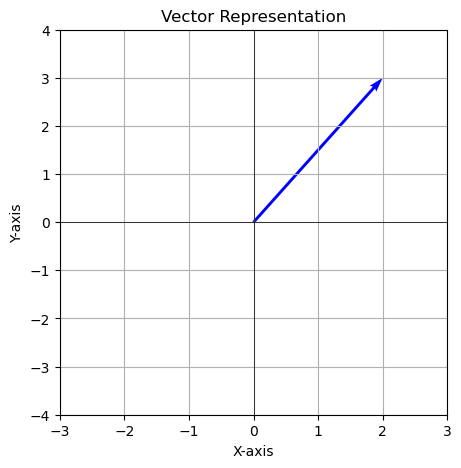
[4]:
import numpy as np
import matplotlib.pyplot as plt

# Define the vector
vector = np.array([2, 3])

# Create the plot
plt.figure(figsize=(5, 5))
plt.quiver(0, 0, vector[0], vector[1], angles='xy', scale_units='xy', scale=1, color='b')
plt.xlim(-3, 3)
plt.ylim(-4, 4)
plt.grid()
plt.axhline(0, color='black',linewidth=0.5)
plt.axvline(0, color='black',linewidth=0.5)
plt.title("Vector Representation")
plt.xlabel("X-axis")
plt.ylabel("Y-axis")
plt.show()
We also know that we can add vectors
and we can also multiply vectors by a constant, or scale the vector
$$ c \vec{v} = 2
=
2.4 Linear Combinations and Spans
A linear combination of two vectors is defined as
Where a and b are scalar values. We call the span of a set of vectors to be a linear combination of those two vectors given an adjustable parameter which are the scalars. The below plot shows an example of the span of vectors \(\vec{u}\) and \(\vec{v}\). The span is of all 2D space indicated by the red dots (imagine these as the end points of vectors)
[7]:
# Define two vectors
vector_u = np.array([1, 2])
vector_v = np.array([2, 1])

# Create a grid of scalar values for the linear combination
scalars = np.linspace(-2, 2, 10)

# Create the plot
plt.figure(figsize=(6, 6))
plt.axhline(0, color='black', linewidth=0.5)
plt.axvline(0, color='black', linewidth=0.5)
plt.grid()

# Plot the span of the vectors
for a in scalars:
    for b in scalars:
        linear_combination = a * vector_u + b * vector_v
        plt.plot(linear_combination[0], linear_combination[1], 'ro', markersize=2)

# Plot the original vectors
plt.quiver(0, 0, vector_u[0], vector_u[1], angles='xy', scale_units='xy', scale=1, color='b', label='Vector u')
plt.quiver(0, 0, vector_v[0], vector_v[1], angles='xy', scale_units='xy', scale=1, color='g', label='Vector v')

plt.xlim(-5, 5)
plt.ylim(-5, 5)
plt.title("Span of Two Linearly Independent Vectors")
plt.xlabel("X-axis")
plt.ylabel("Y-axis")
plt.legend()
plt.show()
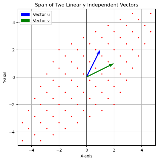
Not all vectors will span 2D space. If both vectors are zero vectors then they will remain at the origin
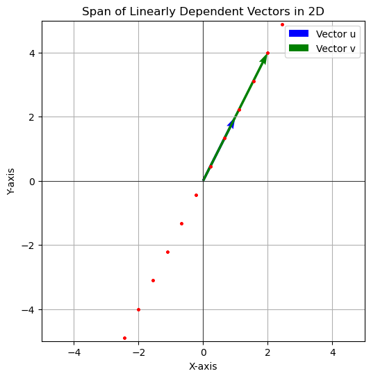
Or, if two vectors are parallel, then the span will only be on the line of the two vectors (as shown below).
[8]:
# Define two linearly dependent vectors
vector_u = np.array([1, 2])
vector_v = 2 * vector_u  # Scalar multiple of vector_u

# Create a grid of scalar values for the linear combination
scalars = np.linspace(-2, 2, 10)

# Create the plot
plt.figure(figsize=(6, 6))
plt.axhline(0, color='black', linewidth=0.5)
plt.axvline(0, color='black', linewidth=0.5)
plt.grid()

# Plot the span of the vectors
for a in scalars:
    for b in scalars:
        linear_combination = a * vector_u + b * vector_v
        plt.plot(linear_combination[0], linear_combination[1], 'ro', markersize=2)

# Plot the original vectors
plt.quiver(0, 0, vector_u[0], vector_u[1], angles='xy', scale_units='xy', scale=1, color='b', label='Vector u')
plt.quiver(0, 0, vector_v[0], vector_v[1], angles='xy', scale_units='xy', scale=1, color='g', label='Vector v')

plt.xlim(-5, 5)
plt.ylim(-5, 5)
plt.title("Span of Linearly Dependent Vectors in 2D")
plt.xlabel("X-axis")
plt.ylabel("Y-axis")
plt.legend()
plt.show()
Review
If you have a set of vectors which does not add dimensionality to the span (i.e. the vectors are parallel in 2D) then it is said that these vectors are linearly dependent. For all other vectors they will be linearly independent. You will see the topic of linear dependence/independence come up when describing a matrix. This description of span and linear dependence/independence also applies to 3D and higher dimensions.
2.5 Matrices
A matrix is a rectangular array of scalar values arranged in rows and columns
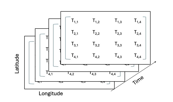
Where \(i\) is the row index and \(j\) is the column index for each element in the matrix. A matrix will have two dimensions listed as MxN. M is the number of rows and N is the number of columns. This will be important when we go into the algebra side. An example of a matrix will be a list or temperature values described by their latitude and longitude position
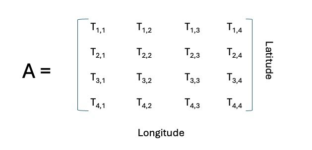
Question: From the above example, what are the dimensions of the 2D matrix (i.e. What is the value for M and N)?
Solution: 4 x 4. Note: A matrix does not have to be a square, it can also be a MxN matrix where M > N or N < M
2.6 Tensors
Scalars, Vectors and Matrices are all different order Tensors. Tensors are described by their order where the order is the description on the number of the dimensions of the object
Scalars are 0th order tensor (a single number)
Vectors are 1st order tensors (a list of numbers [x y z])
Matrices are 2nd order tensors ([M] rows and [N] columns)
There are also 3rd order tensors. An example of this is a tensor with dimensions Latitude x Longitude x Time.
There can also be higher order tensors but for our purposes we will only be using 2nd order tensors (a matrix).
_Note: The definition of the word tensor is a bit confusing because it depends on the field you are in to determine it’s definition.