Integrals
Instructor: Sophie Wynn, Climate Science PhD Student (srwynn@ucsd.edu)
TAs: Luisa Watkins (l1watkins@ucsd.edu) and Lauren Harvey (lrharvey@ucsd.edu)
This lecture introduces integration and covers Riemann Sums, the FTC, and integration by parts.
Lecture Notes inspired by Luisa Watkins and 3Blue1Brown.
1 | Integration
The integral measures the total accumulation of a quantity over time, space etc. For example an integral can compute area, distance, volume, mass, work etc!
To get an understanding of what this means, let’s go through an example:
1.1 Traveling in a Car
Suppose our velocity is given by:
But we were only keeping track of the velocity every second.
Sampled values of velocity
Time (t) (s) |
Velocity (v(t)) (m/s) |
|---|---|
0 |
0 |
1 |
7 |
… |
|
4 |
16 |
8 |
0 |
Question: How far did the car travel between (t = 0) and (t = 8)?
We’ll compute the distance traveled in two ways:
Using a table of sampled values and Riemann sums.
Using the exact integral.
[3]:
import numpy as np
import matplotlib.pyplot as plt

def u(t):
    return t * (8 - t)

time_samples = np.array([0, 1, 4, 8])
u_samples = u(time_samples)

t_cont = np.linspace(0, 8, 400)
u_cont = u(t_cont)

#  Left-Riemann sum setup
dt = 1
t_left = np.arange(0, 8, dt)   # left endpoints: 0,1,2,...,7
u_left = u(t_left)

# Compute left Riemann sum
areas = u_left * dt
total_left_riemann = np.sum(areas)

plt.figure(figsize=(12,5))


# plot continuous velocity curve
plt.plot(t_cont, u_cont, "b-", linewidth=2, label=r"$u(t) = t(8-t)$")

# plot left endpoints
plt.scatter(t_left, u_left, color="red", zorder=5, label="Left endpoints")

# draw rectangles
for i in range(len(t_left)):
    plt.bar(t_left[i], u_left[i], width=dt, align="edge",
            alpha=0.35, edgecolor="k", color="skyblue")

plt.title(f"Left-Riemann Sum (Δt=1)")
plt.xlabel("Time (s)")
plt.ylabel("Velocity $v(t)$ (m/s)")
plt.grid(True)
plt.legend()
plt.tight_layout()
plt.show()
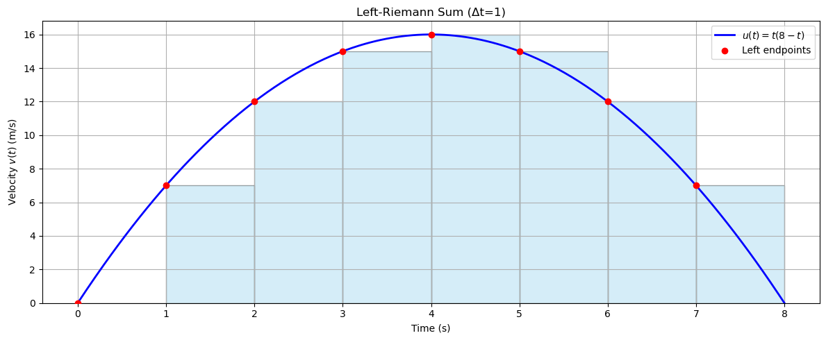
1.2 Riemann Sum
The area of each rectangle is base × height.
The base is \((\Delta t = 1)\) ie (s).
The height is the velocity ie (m/s) at the left endpoint of each interval.
Thus the area will give us meters
So, we can sum up the areas of all rectangles to get an approximation of the total distance traveled.
If we divide the interval into equal parts of width \((\Delta t)\), the Riemann sum is:
where \((t_i)\) is the left endpoint of each interval.
1.3 Car example (with Δt = 1)
Substitute \(v(t) = t(8-t)\):
So, the left Riemann sum approximation of the total distance is:
Imagine if, instead of using a finite \(\Delta t = 1\) second, we could measure the velocity at every instant in time. Then our rectangles would get smaller and smaller, and the sum of their areas would converge to the exact distance traveled!! This is exactly what integration allows us to do.
2 | Introducing the Integral
If we let the intervals become infinitely small (\(\Delta t \to 0\)), the Riemann sum converges to the exact total accumulation, which is written as an integral:
Where:
\(\int\) is the integration operator,
\(a\) and \(b\) are the lower and upper bounds of the interval,
\(f(t)\) is the function being accumulated,
\(dt\) represents an infinitesimally small change in the independent variable.
2.1 Applying to our car example
For the car’s velocity \(v(t)\) from \(t = 0\) to \(t = 8\) s:
The distance traveled is:
Using the exact integral, we get:
So, the true of the total distance is:
This shows how letting \(\Delta t \to 0\) turns the approximation into the true value.
2.2 Computing the Integral
To compute an integral we take the antiderivative of the function and then compute the bounds (if stated).
2.2.1 Step 1: Expand the function
2.2.2 Step 2: Apply the Power Rule for Integration
Recall the power rule, from derivatives, the same rule applies integration but in reverse:
Apply it to each term:
This is the antiderivative \(F(t)\).
2.2.3 Step 3: Evaluate at the Bounds (Fundamental Theorem of Calculus)
The Fundamental Theorem of Calculus says:
Compute:
2.3 The Fundamental Theorem of Calculus
The FCT is key to understanding derivatives and antiderivatives!
In our example, \(F(t) = 4t^2 - \frac{t^3}{3}\) also represents the path function, commonly written as \(x(t)\) in physics or calculus.
Recall from derivatives:
which says the derivative of the path gives the velocity.
Here, we went in the opposite direction: starting from velocity \(v(t)\), we computed the integral to recover the path \(x(t)\).
In other words:
Derivative: path \(\to\) velocity
Integral: velocity \(\to\) path
This shows how integration accumulates small changes in velocity over time to give the total displacement, just like summing the tiny rectangles in a Riemann sum.
Thus, derivatives and integrals are inverse operations, and the Fundamental Theorem of Calculus makes this connection precise.
Derivative: \(v(t) = \frac{dx}{dt}\)
Integral: \(x(b) - x(a) = \int_a^b v(t) \, dt\)
3.1 Power Rule
For \(n \neq -1\):
3.2 Exponential Functions
3.3 Logarithmic Function
3.4 Sine and Cosine
3.5 Other Trigonometric Functions
3.6 Linear Combination Rule
If \(f(x)\) and \(g(x)\) are integrable and \(a,b\) are constants:
3.7 Integration by Substitution (u-substitution)
Used for composite functions:
Example:
3.8 Inverse Trigonometric Functions
3.9 Hyperbolic Functions
3.10 Special Rules / Tricks
Constant Multiple Rule: \(\int a f(x)\, dx = a \int f(x)\, dx\)
Sum/Difference Rule: \(\int (f(x) \pm g(x)) \, dx = \int f(x) dx \pm \int g(x) dx\)
3.11 Integration by Parts
For functions made up of two factors, the integration by parts formula states that for functions \(u(x)\) and \(v(x)\) that are differentiable:
\(u(x)\): function we differentiate
\(v'(x)\): function we integrate
3.11.1 Example
Suppose we want to compute:
Choose parts:
Let \(u(x) = x \quad \Rightarrow \quad u'(x) = 1\)
Let \(v'(x) = \sin(kx) \quad \Rightarrow \quad v(x) = -\frac{1}{k} \cos(kx)\)
Apply the formula:
Substitute:
Simplify:
Integrate remaining term:
So the final result:
Practice Problems
Question 1:
Express velocity \(v\) , at time \(t_1\) , in terms of \(v\) at \(t_0\) and acceleration \(a(t)\)
Question 2:
Find the mass \((m)\) of the container described belowe in terms of density (\(\rho\)) using the fact that \(m =\int \rho dV\)
The container is:
1 m long
3 m tall
Width changes with height (z) as: \(w(z) = (z + 1)^2\)
The container has a constant density (\(\rho\))
Question 3:
Calculate: