Limits and Derivatives

Instructor: Isidora Rojas (i1rojas@ucsd.edu)

TAs: Joey Carter (j6carter@ucsd.edu) and Lauren Harvey (lrharvey@ucsd.edu)

Learning Objectives

• Explain a limit and use it to define the derivative

• Compute derivatives using power, product, quotient, and chain rule

• Understand and identify different forms of differnetiation notation

• Apply derivative rules to oceanographic problems

1 | Limits

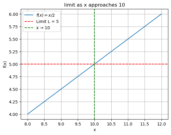
We say that the limit of $ f(x) $ is \(L\) as \(x\) approaches \(a\) and write this as:

\[\lim_{x \to a} f(x) = L\]

This means we can make \(f(x)\) as close to \(L\) as we want for all \(x\) sufficiently close to \(a\), from both sides, without actually letting \(x\) be \(a\).

Simple Example:

\[\lim_{x \to 10} \frac{x}{2} = 5\]

import numpy as np
import sympy as sp
import matplotlib.pyplot as plt

x = np.linspace(8, 12, 200)
y = x/2

plt.plot(x, y, label="$f(x) = x/2$")
plt.axhline(5, color="red", linestyle="--", label="Limit L = 5")
plt.axvline(10, color="green", linestyle="--", label="x → 10")
plt.legend()
plt.xlabel("x")
plt.ylabel("f(x)")
plt.grid(True)
plt.title("limit as x approaches 10")
plt.show()

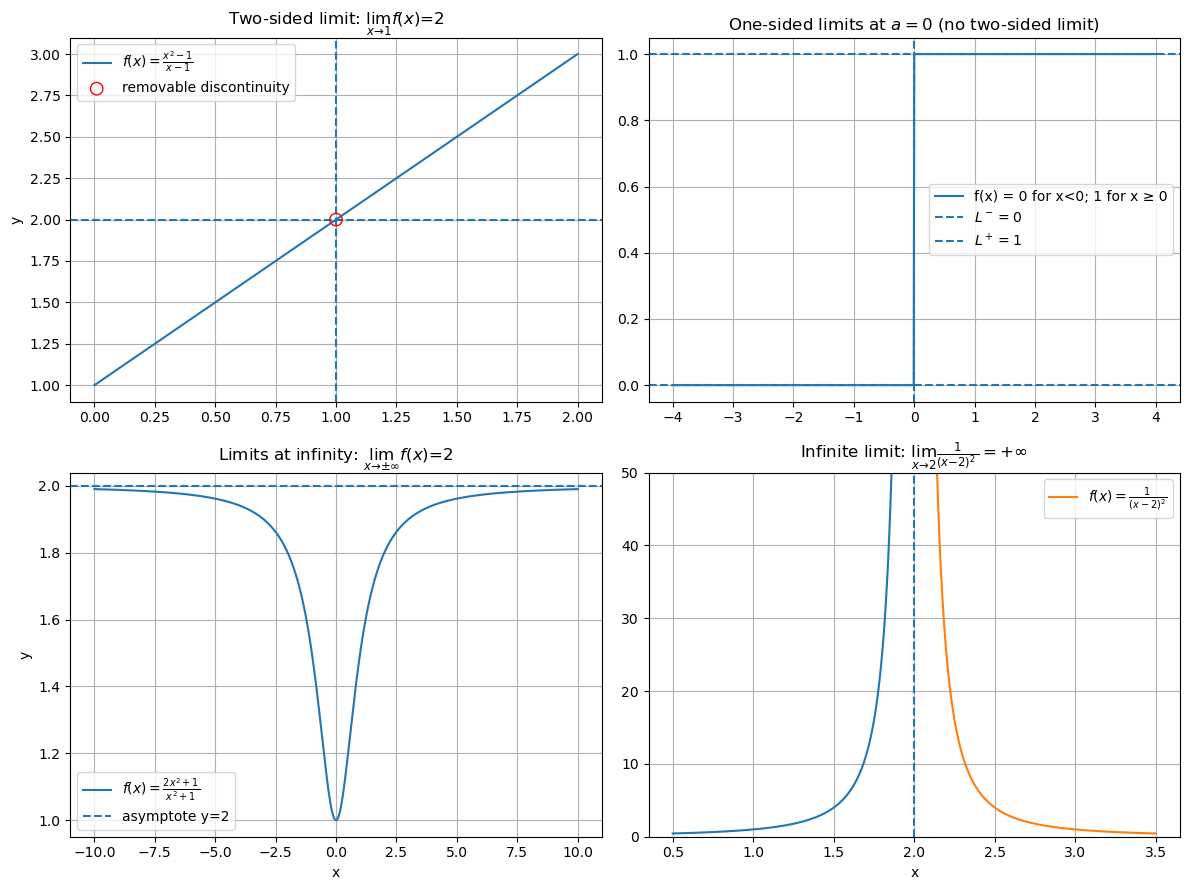
1.1 Kinds of Limits

Note: this will not be covered during workshop time but is intended to be used as a reference

1. Two-sided limit

   \(\lim_{x \to a} f(x) = L\) Requires \(f(x)\) to approach the same \(L\) from both the left (\(x \to a^-\)) and the right (\(x \to a^+\)).

2. One-sided limits

   • Left-hand limit: \(\lim_{x \to a^-} f(x) = L\)

   • Right-hand limit: \(\lim_{x \to a^+} f(x) = L\)

3. Limits at infinity

   • \(\lim_{x \to \infty} f(x)\)

   • \(\lim_{x \to -\infty} f(x)\) Used to describe asymptotic behavior.

4. Infinite limits

   • \(\lim_{x \to a} f(x) = \infty\) Means \(f(x)\) grows without bound as \(x\) approaches \(a\).

---

fig, axes = plt.subplots(2, 2, figsize=(12, 9))

# two-sided limit:
ax = axes[0, 0]
a = 1.0
x = np.linspace(0, 2, 600)
y = (x**2 - 1) / (x - 1)           # equals x+1 for x != 1
y[np.isclose(x, a, atol=1e-6)] = np.nan  # hide the undefined point
ax.plot(x, y, label=r"$f(x)=\frac{x^2-1}{x-1}$")
ax.axvline(a, linestyle="--")                 # approach point
ax.axhline(2, linestyle="--")                 # limit value
ax.scatter([a], [2], facecolors="none", edgecolors="red", s=80, zorder=3,
           label="removable discontinuity")
ax.set_title("Two-sided limit: $\\lim_{x\\to 1} f(x) = 2$")
ax.grid(True)
ax.legend(loc="best")

# one-sided limits: step (different left/right limits at a=0)
ax = axes[0, 1]
a = 0.0
x = np.linspace(-4, 4, 801)
f = np.where(x < 0, 0.0, 1.0)
ax.plot(x, f, label="f(x) = 0 for x<0; 1 for x ≥ 0")
ax.axvline(a, linestyle="--")
ax.axhline(0, linestyle="--", label=r"$L^- = 0$")
ax.axhline(1, linestyle="--", label=r"$L^+ = 1$")
ax.set_title("One-sided limits at $a=0$ (no two-sided limit)")
ax.grid(True)
ax.legend(loc="best")

# limits at infinity- horizontal asymptote
ax = axes[1, 0]
x = np.linspace(-10, 10, 1201)
f = (2*x**2 + 1) / (x**2 + 1)
ax.plot(x, f, label=r"$f(x)=\frac{2x^2+1}{x^2+1}$")
ax.axhline(2, linestyle="--", label="asymptote y=2")
ax.set_title(r"Limits at infinity: $\lim_{x\to\pm\infty} f(x)=2$")
ax.grid(True)
ax.legend(loc="best")

# infinite limit at a point: vertical asymptote
#    f(x) = 1/(x-2)^2 -> +∞ as x -> 2
ax = axes[1, 1]
a = 2.0

x_left  = np.linspace(0.5, 1.95, 400)
x_right = np.linspace(2.05, 3.5, 400)
f_left  = 1.0 / (x_left - a)**2
f_right = 1.0 / (x_right - a)**2
ax.plot(x_left, f_left)
ax.plot(x_right, f_right, label=r"$f(x)=\frac{1}{(x-2)^2}$")
ax.axvline(a, linestyle="--")                 # vertical asymptote
ax.set_ylim(0, min(50, max(f_left.max(), f_right.max())))  # keep plot readable
ax.set_title(r"Infinite limit: $\lim_{x\to 2} \frac{1}{(x-2)^2}=+\infty$")
ax.grid(True)
ax.legend(loc="best")

for ax in axes[1, :]:
    ax.set_xlabel("x")
for ax in axes[:, 0]:
    ax.set_ylabel("y")

plt.tight_layout()
plt.show()

2 | Derivatives

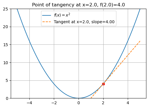
The derivative represents the instantaneous rate of change of a function.

• Secant slope = average rate of change between two points.

• Tangent slope = instantaneous rate of change.

Definition of derivative:

\[f'(x) = \lim_{h \to 0}\frac{f(x+h) - f(x)}{h}\]

import numpy as np
import matplotlib.pyplot as plt
#import ipywidgets as widgets

f = lambda x: x**2
df = lambda x: 2*x

x = np.linspace(-5, 5, 400)
y = f(x)

#@widgets.interact(x0=(-4.0, 4.0, 0.1))
#def tangent_plot(x0=1):
plt.figure(figsize=(6,4))
plt.plot(x, y, label="$f(x) = x^2$")
plt.scatter([x0], [f(x0)], color="red")
plt.ylim(0,25)
plt.title(f"Point of tangency at x={x0}, f({x0})={f(x0)}")

# tangent line
slope = df(x0)
tangent = slope*(x - x0) + f(x0)
plt.plot(x, tangent, "--", label=f"Tangent at x={x0}, slope={slope:.2f}")
plt.ylim(0, 25)

plt.legend()
plt.grid(True)
plt.show()

2.1 Derivative Rules Cheat Sheet

• Power Rule: \(\frac{d}{dx}[x^n] = nx^{n-1}\)

• Constant Rule: \(\frac{d}{dx}[c] = 0\)

• Sum Rule: \(\frac{d}{dx}[f+g] = f' + g'\)

• Product Rule: \(\frac{d}{dx}[fg] = f'g + fg'\)

• Quotient Rule: \(\frac{d}{dx}\left[\frac{f}{g}\right] = \frac{f'g - fg'}{g^2}\)

• Chain Rule: \(\frac{d}{dx}[f(g(x))] = f'(g(x)) \cdot g'(x)\)

• Exponential: \(\frac{d}{dx}[e^x] = e^x\), \(\;\;\frac{d}{dx}[a^x] = a^x\ln(a)\)

• Logarithm: \(\frac{d}{dx}[\ln(x)] = \frac{1}{x}\)

• Trigonometric: \(\frac{d}{dx}[\sin(x)] = \cos(x)\), \(\frac{d}{dx}[\cos(x)] = -\sin(x)\), \(\frac{d}{dx}[\tan(x)] = \sec^2(x)\)

2.2 Useful Derivatives

\(\frac{d}{dx}(x) = 1\)

\(\frac{d}{dx}(\sin x) = \cos x\)

\(\frac{d}{dx}(\cos x) = -\sin x\)

\(\frac{d}{dx}(\tan x) = \sec^2 x\)

\(\frac{d}{dx}(\cot x) = -\csc^2 x\)

\(\frac{d}{dx}(\sec x) = \sec x \tan x\)

\(\frac{d}{dx}(\csc x) = -\csc x \cot x\)

\(\frac{d}{dx}(\sin^{-1} x) = \frac{1}{\sqrt{1-x^2}}\)

\(\frac{d}{dx}(\cos^{-1} x) = -\frac{1}{\sqrt{1-x^2}}\)

\(\frac{d}{dx}(\tan^{-1} x) = \frac{1}{1+x^2}\)

\(\frac{d}{dx}(\ln(x)) = \frac{1}{x}, \; x > 0\)

\(\frac{d}{dx}(\ln|x|) = \frac{1}{x}, \; x \neq 0\)

\(\frac{d}{dx}(\log_a(x)) = \frac{1}{x \ln(a)}, \; x > 0\)

\(\frac{d}{dx}(e^x) = e^x\)

\(\frac{d}{dx}(a^x) = a^x \ln(a)\)

2.3 Derivative Notation

There are several common notations for derivatives:

Notation Type	Example	Context
Lagrange	\(f'(x), f''(x)\)	General functions
Leibniz	\(\frac{dy}{dx}, \frac{d^2y}{dx^2}\)	Differential equations, rigor
Newton	\(\dot{y}, \ddot{y}\)	Physics, time derivatives
Euler	\(Df(x)\)	Operator form
Partial	\(\frac{\partial f}{\partial x} , \frac{\partial^2 f}{\partial x^2}\)	Multivariable calculus

Practice Problems

Using the derivative rules (power, product, quotient, chain, exponential, logarithmic, trigonometric), solve the following:

1. What is the instantaneous rate of change at \(x=2\) of \(f(x)=\frac{x^2-2}{x-1}\)

solution:

Steps

• Use the quotient rule: if \(f=\dfrac{u}{v}\) then \(f'=\dfrac{u'v-uv'}{v^2}\) with \(u=x^2-2\), \(v=x-1\).

• Compute \(u'=2x\), \(v'=1\).

• Substitute and simplify, then evaluate at \(x=2\).

• Work \(,f'(x)=\dfrac{(2x)(x-1)-(x^2-2)(1)}{(x-1)^2} =\dfrac{x^2-2x+2}{(x-1)^2}.\) So \(,f'(2)=\dfrac{4-4+2}{1}=2.\)

x = np.linspace(1.5, 2.5, 1000)
f = (x**2 - 2) / (x - 1)

# compute derivative
dfdx = np.gradient(f, x)

# solve at x=2
x0 = 2.0
idx = (np.abs(x - x0)).argmin()
print("f'(2) ≈", dfdx[idx])

f'(2) ≈ 1.9990007500003912

2. What is the derivative on \(sin(e^{-x})\)?

solution:

• Let \(u=e^{-x}\). Use the chain rule: \((\sin u)'=\cos u\cdot u'\).

• Compute \(u'=-e^{-x}\).

x = sp.symbols('x')
f = sp.sin(sp.exp(-x))
dfdx = sp.diff(f, x)
print("f(x) = ", f)
print("f'(x) =", dfdx)

f(x) =  sin(exp(-x))
f'(x) = -exp(-x)*cos(exp(-x))

3. What is the derivative of $ \frac{d^2}{dx^2} e^{ix}$, where \(i=\sqrt{-1}\)?

solution:

• First derivative by chain rule: \((e^{ix})'=i,e^{ix}\).

• Differentiate again: \((i,e^{ix})'=i(i,e^{ix})=i^2 e^{ix}=-e^{ix}\).

x = sp.symbols('x')
f = sp.exp(sp.I*x)
dfdx = sp.diff(f,x)
d2fx2 = sp.diff(dfdx,x)

print("f(x) =", f )
print("f '(x) =", dfdx)
print("f''(x) =", d2fx2)

f(x) = exp(I*x)
f '(x) = I*exp(I*x)
f''(x) = -exp(I*x)

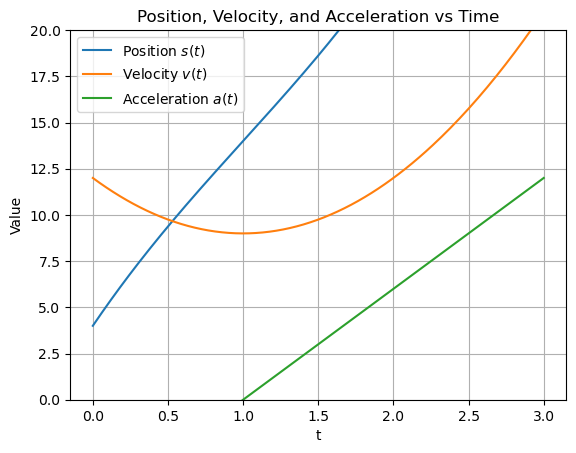
4. What is the max acceleration on interval $ 0 \le `t :nbsphinx-math:le 3`$ if a particle’s position is given by $$ s(t) = t^3 - 3t^2 + 12t + 4?

solution:

• Velocity: \(v(t)=s'(t)=3t^2-6t+12\).

• Acceleration: \(a(t)=v'(t)=6t-6\).

• To maximize \(a\) on a closed interval, check critical points of \(a\) (solve \(a'(t)=0\)) and the endpoints \(t=0,3\).

• Here \(a'(t)=6>0\) (no interior extrema), so \(a\) is increasing; max occurs at the right endpoint.

t = sp.symbols('t')
s = t**3 - 3*t**2 + 12*t + 4

v = sp.diff(s, t)
a = sp.diff(v, t)

s_func = sp.lambdify(t, s, 'numpy')
v_func = sp.lambdify(t, v, 'numpy')
a_func = sp.lambdify(t, a, 'numpy')

t_vals = np.linspace(0, 3, 200)
s_vals = s_func(t_vals)
v_vals = v_func(t_vals)
a_vals = a_func(t_vals)

max_accel = a_vals.max()

print("Max acceleration on [0,3]:", max_accel)

Max acceleration on [0,3]: 12.0

plt.plot(t_vals, s_vals, label="Position $s(t)$")
plt.plot(t_vals, v_vals, label="Velocity $v(t)$")
plt.plot(t_vals, a_vals, label="Acceleration $a(t)$")

plt.xlabel("t")
plt.ylabel("Value")
plt.ylim(0, 20)
plt.title("Position, Velocity, and Acceleration vs Time")
plt.legend()
plt.grid(True)
plt.show()

5. A wave height is given by \(H(t) = \sin(2t)\). Find the rate of change of height at \(t = \pi/6\).

solution:

• Differentiate: \(H'(t)=2\cos(2t)\) (chain rule).

• Plug in \(t=\pi/6\): \(2t=\pi/3\), \(\cos(\pi/3)=1/2\).

❗ Bonus Question: Mean Girls limit problem ❗

Solve the question asked to Cady Heron at the end of Mean Girls:

Hint: L’hopital’s rule:

\[\lim_{x \to a} \frac{f(x)}{g(x)} = \lim_{x \to a} \frac{f'(x)}{g'(x)}\]

solution:

LIMIT DOES NOT EXIST